Building a crown closure model from satellite data

The problem

Crown closure is a useful forest structure signal. It can help identify where dense canopy exists, where there is non-forest, and where downstream models may need different inputs. One important use case is wildfire behavior modelling, where forest density and canopy structure affect how fire can spread through undergrowth and into the canopy.

The task was to produce a pixel-wise prediction over 256 by 256 image chips. Each output pixel represented a value from 0 to 100: the estimated crown closure percentage for that area.

That sounds simple, but the real challenge was that this was not a normal image task. The input was not a single RGB image. It was a carefully aligned stack of satellite and terrain layers, each with its own resolution, timestamp, projection, and metadata. The output also had to be geospatially meaningful, not just visually plausible.

Building the input data cube

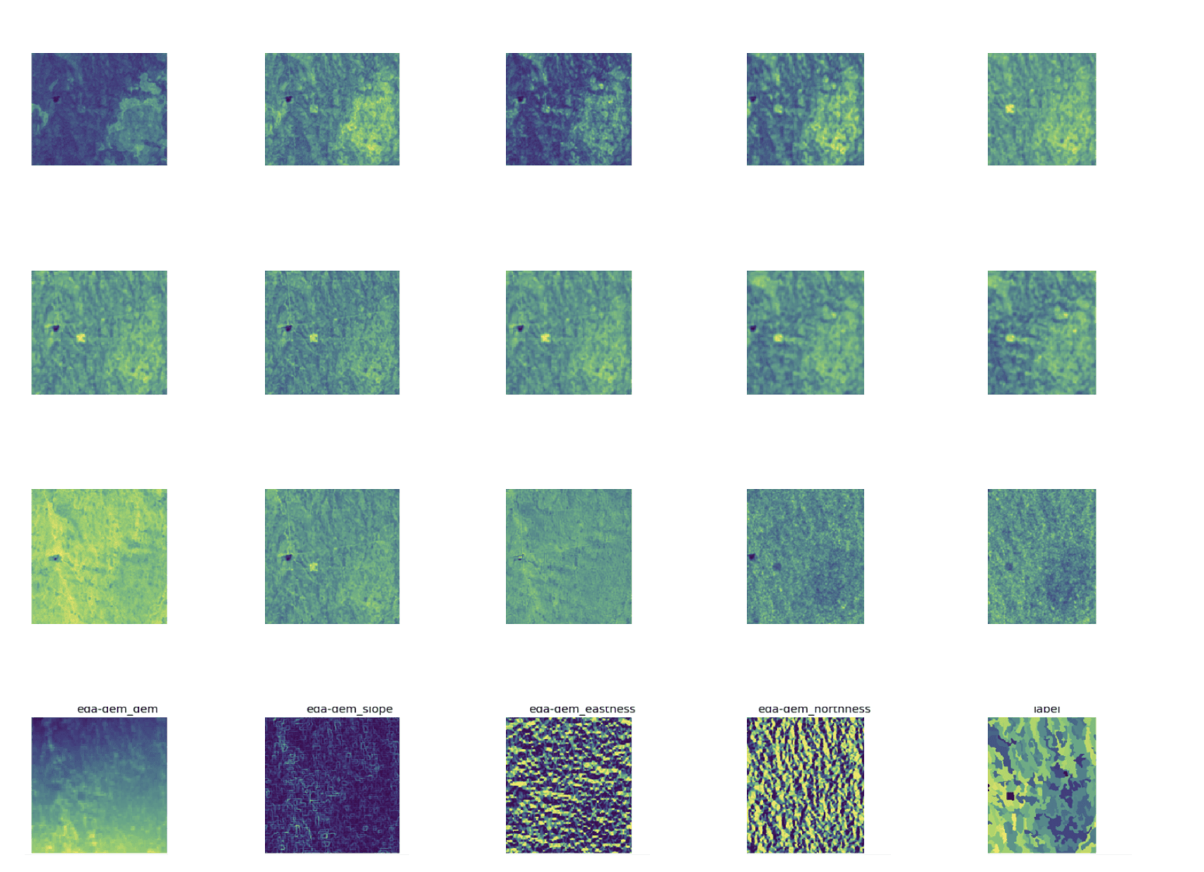
The model used a fusion of multiple satellite products and derived variables. I worked with optical bands such as red, green, blue, near infrared, and short-wave infrared, along with vegetation indices like NDVI. I also used synthetic aperture radar, which is useful because it can provide signal even when optical imagery is limited by clouds.

Terrain also mattered. Elevation, slope, and aspect can affect where different kinds of forest grow. One subtle issue with aspect is that it is circular: 359 degrees and 0 degrees both represent nearly the same direction, but a model can treat them as far apart. To make that easier to learn, I represented aspect through eastness and northness features instead of a raw 0 to 360 degree value.

Before building the final system, I spent time on a literature review of crown closure and related forest-structure prediction work. That helped guide choices around preprocessing, satellite sources, model architectures, loss functions, and validation strategies. It also made the project feel less like guessing and more like engineering from prior evidence.

Working with imperfect truth data

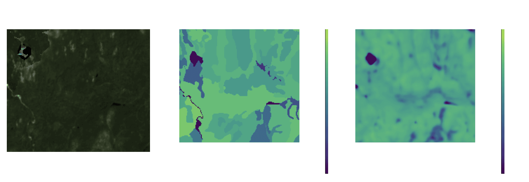
The training labels came from the National Forest Inventory of Canada, which contains expert-labeled forest plots across the country. Those labels were valuable, but they were not perfect. Some polygons were coarse, some water boundaries were imprecise, and some labels were older than the satellite imagery.

Time alignment became one of the biggest constraints. Sentinel-2 imagery for Canada started in 2017, but some label data predated that. Forests change over time, so using old labels against newer imagery introduced error the model could not learn away. Filtering to better-aligned data reduced the dataset substantially, but it made the signal cleaner.

That filtering removed a large portion of the original labels, but it improved the quality of the learning problem. Even with fewer chips, each example still contained 256 by 256 dense pixel labels. In a different modelling context, that could be thought of as many millions of supervised pixel observations rather than only a small number of files.

There was also a waiting problem. The real NFI data took time to obtain, so I created mock training data to keep the project moving. I reverse engineered a downstream wall-to-wall forest product into polygon-like labels that resembled the eventual format. It was not the final truth source, but it let me build and test the preprocessing and training pipeline before the real labels arrived.

Scaling geospatial preprocessing

The ingestion pipeline had to combine many geospatial layers: optical bands, infrared bands, SAR, derived vegetation indices, elevation, slope, aspect, and labels. With geospatial data, small metadata mistakes can corrupt the entire dataset, so I wrote and fixed tests around coordinate reference systems, timestamps, missing values, duplicate records, and expected uniqueness.

I also ran into a scaling problem. The existing ingestion path was not shaped for thousands of dispersed chips, and the work started behaving poorly as the number of regions grew. I split ingestion into many smaller AWS Batch jobs so each job handled a manageable subset of chips. That made the pipeline more practical and resilient.

The scaling issue came from the way the internal pipeline searched for polygons inside each region. My data was already organized as many small, dispersed areas, so feeding all of it through one large run made the search pattern behave badly. Splitting the work into batches, such as many jobs with a small number of chips each, avoided the worst of that growth.

I learned that data preprocessing for satellite imagery has to be treated like production software. Coordinate reference systems, transforms, timestamps, duplicates, null values, and uniqueness constraints all matter. If one metadata field is wrong, the model can train on data that looks valid but is spatially misaligned.

I used AWS Batch and EC2-based workflows for ingestion and training. Because spot instances are much cheaper but can terminate unpredictably, the pipeline needed to fail gracefully and resume from saved progress. Intermediate outputs were written as chunks so a failed job did not mean starting the entire ingestion run again.

Training and validation

The model was a PyTorch U-Net with roughly 32 million parameters. Although the filtered dataset had far fewer chips than the full inventory, each chip contained dense pixel-level supervision. I tested scale-ups from small subsets to larger sets and watched for diminishing returns to make sure the model was still learning useful structure.

One challenge was that the data distribution was heavily imbalanced: many pixels had zero crown closure. The model became conservative in forested regions and produced blurry boundaries around lakes and forest edges. Moving from squared-error style losses toward mean absolute error helped reduce that blurriness and produced sharper prediction chips.

I tried several approaches before landing there. Removing fully non-forest chips seemed reasonable, but it did not solve the core problem. Reweighting forest-heavy chips in the loss function also did not produce the improvement I wanted. The most useful change was moving away from a loss that strongly punished large errors and pushed the model toward safe, blurry midpoint predictions.

This was a case where the metric and the visual output had to be interpreted together. A model can look decent on aggregate error while still making predictions that are too fuzzy around forest boundaries. For crown closure, those boundaries matter because the product is supposed to support downstream spatial reasoning.

Comparing against external products

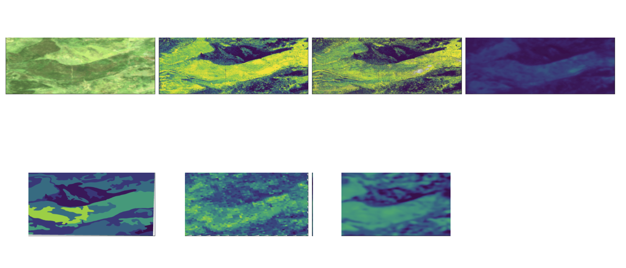
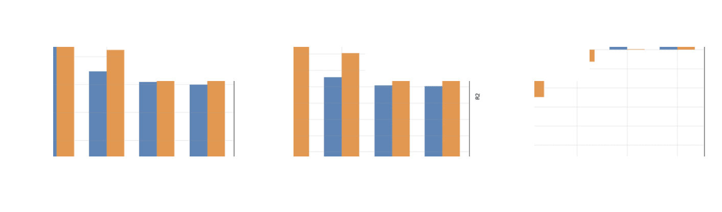
Validation was not only about comparing predictions to the same labels used during training. We also looked at external validation sources, including lidar-derived measurements for specific regions. Lidar is not always available at the scale needed for training, but where it exists it can be a strong validation signal.

I compared the in-house U-Net model against existing crown closure products, including SCANFI. The goal was to understand not only whether my model could fit the NFI labels, but whether it produced a better product when checked against independent data. This was especially important because the training labels themselves had known imperfections.

The model performed strongly in those comparisons, but I also had to be honest about tradeoffs. A U-Net can be more expensive than simpler tree-based approaches. In remote sensing, that tradeoff matters because wall-to-wall maps at fine resolution can involve enormous amounts of data.

What I took away

This internship taught me how different applied ML feels when the hardest problems are not only model architecture. The real work was often in truth-data quality, time alignment, geospatial metadata, preprocessing reliability, and validation against external data.

It also made me much more comfortable working in a large codebase: writing focused bug fixes, reviewing pull requests, running ingestion on AWS, and building tests for data pipelines where one broken metadata field can quietly ruin everything downstream.

The project also taught me how to communicate technical work in a structured engineering environment. We had standups, sprint planning, retrospectives, reviews, and periodic presentations. I had to explain not only what the model was doing, but why certain data decisions mattered and how they affected the final product.

Looking back, the most valuable part was learning to treat applied ML as a full system. The model was only one piece. The quality of the result depended on data contracts, scalable ingestion, geospatial correctness, validation design, and careful iteration under real-world constraints.